Beginner Tutorial

This tutorial will cover:

• Downloading OrthoFinder
• Running OrthoFinder
• Exploring the results of OrthoFinder

OrthoFinder requires as input the amino acid sequences for all the protein coding genes in your species of interest. We provide a separate tutorial for getting input files for OrthoFinder.

All these steps will be done on the command line so that you can just copy and paste the commands yourself. If you are not familiar with the command line there are many online tutorials and reference pages, here is a nice short one that covers the basics.

Downloading OrthoFinder

There are two main ways of getting OrthoFinder. You can either use conda, or you can install it directly from GitHub. Installing directly from GitHub will always give you the latest version, but you might have to manually install other software that OrthoFinder is dependent on, and it can be trickier to troubleshoot if you aren’t familiar with the command line. Conda automates the installation process and handles all dependencies, making it very beginner-friendly. To install via conda, we first need to install miniconda. Follow the instructions here.

We then need to run these commands

conda config --add channels defaults conda config --add channels bioconda conda config
--add channels conda-forge
conda create -n orthofinder
conda activate orthofinder
conda install orthofinder

If you are on one of the newer Macs with the new chips (M1/M2/M3), you might need to follow a few extra steps to use conda. Check out the guide here.

To install directly from GitHub, we need to run these commands

python3 -m venv of3_env
. of3_env/bin/activate
pip install git+https://GitHub.com/OrthoFinder/OrthoFinder.git

You can test that OrthoFinder has been installed by printing its help file orthofinder -h, which will print all of the command line options.

You can test that OrthoFinder is working correctly by running it on the example dataset, which you can download from our GitHub

orthofinder -f ExampleData/

OrthoFinder will print lots of information to the command line as it runs. If you get an error message, the best way to troubleshoot is to just google the error message. You can also ask a question on our GitHub.

When OrthoFinder has finished running, it will generate a folder containing the output, with the folder named according to today’s date. ExampleData/OrthoFinder/Results_Jul12 The folder looks like this:

We’ll discuss how to interpret and analyse these files and folders later on, in the Exploring the results section of the tutorial.

Running OrthoFinder

You can now run OrthoFinder First, you have to open a terminal and navigate to the directory where your files are. You can now run OrthoFinder on your proteomes.

orthofinder -f primary_transcripts 

That’s it! OrthoFinder will print updates on its progress to the terminal, and tell you when it’s finished. To see what options you might want to adjust for your own data, check out the GitHub, or the Advanced Tutorial page

Exploring the results of OrthoFinder

OrthoFinder creates a results directory named OrthoFinder inside the proteome directory, and puts the results here. My results directory looks like this:

Step 1: Quality Control

Before we start diving into the orthogroups, it would behoove us to check the quality of the OrthoFinder run. We want to make sure that most genes across all species have been assigned to orthogroups, and that the species tree looks realistic.

Open the file Statistics_Overall.tsv from the folder Comparative_Genomics_Statistics. This file can be opened in spreadsheet software like Microsoft Excel, or in a text editor like Notepad.

On the 5th line, we can see the ‘Percentage of genes in orthogroups’, which in my case is 95.7%.

A good rule of thumb is that this number should be >80%. If not, you are likely missing some orthology relationships that actually exist. The best way to fix this would be better species sampling.

Now open the file ‘Statistics_PerSpecies’, from the same folder. This file gives us the % of genes in each species that are assigned to orthogroups, rather than the percentage for all genes across species.

You can see here that we capture most genes across all species.

The lowest percentage is the kiwi (A. haastii), but we still managed to assign 94% of its genes to orthogroups. The key message here is that it’s always a good idea to look at this information before you start interpreting your results. If the numbers were too low for one species, we might want to consider sampling more species to fill in the long evolutionary divergence between species (e.g. something in between a Kiwi and a Kakapo, such as a Hoatzin).

One more useful thing to do before we really start to dive in is to look at the species tree. Go to the iTOL website, and click Upload a tree. You can then drag and drop the tree file, which is in Species_Tree/SpeciesTree_rooted.txt You will now see the phylogenetic tree that OrthoFinder has produced. I have annotated my version with icons PhyloPic, so that we can see what is going on

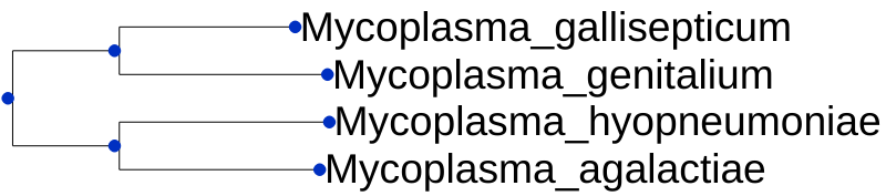
We now want to do some common-sense checking that everything appears to be in order, and we aren’t rewriting the history of life on earth. With our six species, this tree looks exactly as we would expect. If the tree doesn’t look correct, then this won’t impact orthogroup inference, but will affect our measures of gene duplication, and might affect our assignment of orthologs and paralogs within an orthogroup. If you need to, you can run OrthoFinder with your own species tree (use the -s option).

Step 2: Interpreting results

Now that we are happy with our OrthoFinder run, we can start diving into the results.

• Orthologues
  We will start by finding orthologues of a gene that we are interested in. We will focus on the gene ENSVURG00010002700.1 in wombats, which is an olfactory receptor. Let’s find out what its orthologues are in the Tammar wallaby. In the Orthologues directory there is a sub-directory for each species.

  Open Orthologues/Orthologues_Vombatus_ursinus/Vombatus_ursinus v Notamacropus_eugeni i.tsv, in a spreadsheet program (specifying that it’s tab-delimited if necessary). The file has three columns, Orthogroup, Vombatus_ursinus, and Notamacropus_eugenii. Find ENSVURG00010002700.1 in the table, I can see that the gene is in orthogroup OG0000365 and that it has three orthologues in wallabies: ENSMEUG00000016785.1, ENSMEUG00000001827.1, ENSMEUG00000010434.1

• Gene trees
  Next, we are going to look at the gene tree to see how these orthologues arose. OrthoFinder infers orthlologues from resolved gene trees using a Duplication-Loss- Coalescence analysis to identify the more parsimonious interpretation of the tree (see the OrthoFinder2 paper for more details).

  All of the gene trees are in one file (Resolved_Gene_Trees/Resolved_Gene_Trees.txt). Each line of the file contains the ID of an orthogroup (e.g. OG0000365:), followed by the gene tree for that orthogroup. To find the tree for certain orthogroup, just search for the orthogroup ID.

  We are going to view the tree for OG0000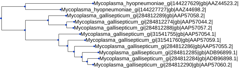365 on iTOL.

  

  Looking at the gene tree, we can see that there have been several gene duplications in the lineage leading to wallabies (Notamacropus). This has resulted in a one-to-three orthology relationship, i.e. all three of the wallaby genes are equally related to the wombat gene ENSVURG00010002700.1. It’s often the case that orthology relationships aren’t one-to-one, and it’s important to know this—you don’t want to spend months doing experiments on ‘the orthologue’ only to find out later there are actually three!

• Gene duplications
  Having the gene trees means that OrthoFinder can identify all gene duplication events that occurred. There is a folder called Gene_Duplication_Events that has two files that allow us to explore duplications. Let’s first open Gene_Duplication_Events/SpeciesTree_Gene_Duplications_0.5_Support.txt in iTOL. Go into the Advanced tab on the Control Panel and select Display next to Node IDs to see the node labels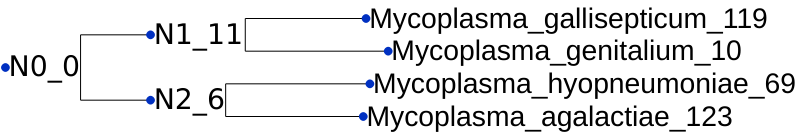

  

  This gives a summary of gene duplication events. Each node shows the node name followed by an underscore and then the number of well-supported gene duplication events mapped to each node in the species tree. Gene-duplication events are considered well-supported if at least 50% of the descendant species have retained both copies of the duplicated gene. For the common ancestor of the mammals, N2, there were 812 of these well-supported gene duplication events. The numbers after the species names are the number of terminal duplications that map to that species, rather than an internal node of the species tree.

  We can see the full list of gene duplication events in the file Gene_Duplication_Events/Duplications.tsv. Here are just a few lines from the file:

  

  Each gene duplication event is cross-referenced to the species tree node, and the node in the gene tree. It also lists the genes descended from each of the two copies arising from the gene duplication event. We can check this out for our wombat olfactory receptor orthologues.

  

  These events are also summarised by orthogroup and by species tree node in the files Duplications_per_Orthogroup.tsv and Duplications_per_Species_Tree_Node.tsv which are both in the directory Comparative_Genomics_Statistics/.

• Orthogroups
  Often we’re interested in group-wise species comparisons, that is comparisons across a clade of species rather than between a pair of species. The generalisation of orthology to multiple species is the orthogroup. Just like orthologues are the genes descended from a single gene in the last common ancestor of a pair of species an orthogroup is the set of genes descended from a single gene in a group of species. Each gene tree from OrthoFinder, for example the one above, is for one orthogroup. The orthogroup gene tree is the tree we need to look at if we want it to include all pairwise orthologues. And even though some of the genes within an orthogroup can be paralogs of one another, if we tried to take any genes out then we would also be removing orthologs too.

  So if we want to do a comparison of the equivalent genes in a set of species, we need to do the comparison across the genes in an orthogroup. The orthogroups are in the file Orthogroups/Orthogroups.tsv. This table has one orthogroup per line and one species per column and is ordered from largest orthogroup to smallest.

• Hierarchical Orthogroups
  OrthoFinder3 also infers hierarchical orthogroups for each node in the species tree. A file equivalent to Orthogroups/Orthogroups.tsv is available for each node in /Phylogenetic_Hierarchical_Orthogroups. You can compare the node number (e.g. N3) to the species tree, to see which species will be included.

• Orthogroup sequences
  For each orthogroup there is a FASTA file in Orthogroup_Sequences/ which contains the sequences for the genes in that orthogroup.

• Other results files
  We have now covered all of the main output files that will be useful to most users, but OrthoFinder also outputs much more useful information! A full description of the output files is available below.

  There are also some useful community tools that allow interactive viewing of results, such as OrthoBrowser